Analysis of the Heart Data Set
%input the data and plot the time series
heart=dlmread('heart.dat');
plot(1:2048, heart, '-')
%look at help for the functions we need
help MakeONFilter
help FWT_PO
help PlotMultiRes
  MakeONFilter -- Generate Orthonormal QMF Filter for Wavelet Transform
   Usage
     qmf = MakeONFilter(Type,Par)
   Inputs
     Type   string, 'Haar', 'Beylkin', 'Coiflet', 'Daubechies',
            'Symmlet', 'Vaidyanathan','Battle'
     Par    integer, it is a parameter related to the support and vanishing
            moments of the wavelets, explained below for each wavelet.

  Outputs
     qmf    quadrature mirror filter

   Description
     The Haar filter (which could be considered a Daubechies-2) was the
     first wavelet, though not called as such, and is discontinuous.

     The Beylkin filter places roots for the frequency response function
     close to the Nyquist frequency on the real axis.

     The Coiflet filters are designed to give both the mother and father
     wavelets 2*Par vanishing moments; here Par may be one of 1,2,3,4 or 5.

     The Daubechies filters are minimal phase filters that generate wavelets
     which have a minimal support for a given number of vanishing moments.
     They are indexed by their length, Par, which may be one of
     4,6,8,10,12,14,16,18 or 20. The number of vanishing moments is par/2.

     Symmlets are also wavelets within a minimum size support for a given
     number of vanishing moments, but they are as symmetrical as possible,
     as opposed to the Daubechies filters which are highly asymmetrical.
     They are indexed by Par, which specifies the number of vanishing
     moments and is equal to half the size of the support. It ranges
     from 4 to 10.

     The Vaidyanathan filter gives an exact reconstruction, but does not
     satisfy any moment condition.  The filter has been optimized for
     speech coding.

     The Battle-Lemarie filter generate spline orthogonal wavelet basis.
     The parameter Par gives the degree of the spline. The number of
     vanishing moments is Par+1.

   See Also
     FWT_PO, IWT_PO, FWT2_PO, IWT2_PO, WPAnalysis

   References
     The books by Daubechies and Wickerhauser.


  FWT_PO -- Forward Wavelet Transform (periodized, orthogonal)
   Usage
     wc = FWT_PO(x,L,qmf)
   Inputs
     x    1-d signal; length(x) = 2^J
     L    Coarsest Level of V_0;  L << J
     qmf  quadrature mirror filter (orthonormal)
   Outputs
     wc    1-d wavelet transform of x.

   Description
     1. qmf filter may be obtained from MakeONFilter
     2. usually, length(qmf) < 2^(L+1)
     3. To reconstruct use IWT_PO

   See Also
     IWT_PO, MakeONFilter


  PlotMultiRes -- Multi-Resolution Display of 1-d Wavelet Transform
   Usage
     PlotMultiRes(wc,L,scal,qmf)
   Inputs
     wc    1-d wavelet transform
     L     level of coarsest scale
     scal  scale factor [0 ==> autoscale]
     qmf   quadrature mirror filter used to make wc

   Side Effects
     A depiction of the multi-resolution decomposition
     of the signal, as in S. Mallat.

   See Also
     PlotWaveCoeff, FWT_PO, IWT_PO, MakeONFilter
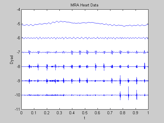
%Use Symmlet 4 (Same as LA8) and J0=6
qmf = MakeONFilter('Symmlet', 8);
wc  = FWT_PO(heart,6,qmf);
PlotMultiRes(wc,6,0,qmf);
title('MRA Heart Data')
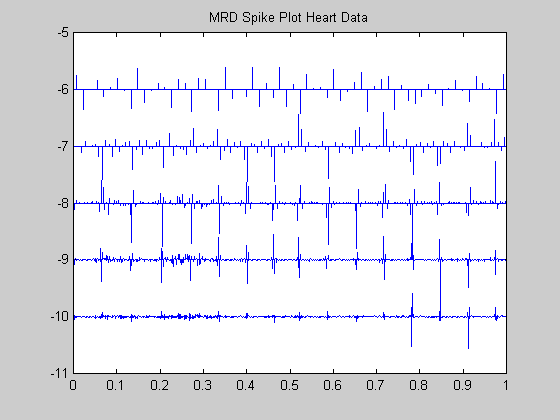
Spike-plot display of wavelet coefficients
PlotWaveCoeff(wc,6,0);
title('MRD Spike Plot Heart Data')
Now we look at the MODWT MRA Analysis
help FWT_Stat
help PlotStatTable
wc = FWT_Stat(heart, 6, qmf);
PlotStatTable(wc,0);
title('MRA Heart Data: MODWT')
  FWT_Stat -- stationary wavelet transform
   Usage
     StatWT = FWT_Stat(x,D,qmf)
   Inputs
     x        array of dyadic length n=2^J
     L        degree of coarsest scale
     qmf      orthonormal quadrature mirror filter
   Outputs
     StatWT   stationary wavelet transform table
              formally same data structure as packet table
              log_2(n)-D scales by n elements

   See Also
     IWT_Stat, FWT_TI


  PlotStatTable -- Plot Stationary Wavelet Transform
   Usage
     PlotStatTable(StatWT,scal)
   Inputs
     StatWT   1-d stationary wavelet transform
     scal     optional scale factor [0 ==> autoscale]

   Side Effects
     A depiction of the stationary wavelet transform,
     much like multi-resolution decomposition
     of signal

   See Also
     PlotMultiRes, FWT_Stat, IWT_Stat
